bits, bytes & numerical sound / part 1
Building an Acoustic Solver from Scratch
This is the first in a series where I document building an FWH acoustic solver, a differentiable, GPU-native tool for predicting flow-induced noise. The choices, the detours, and what I learn along the way.
This project is also a means of learning and applying a bunch of ideas to see how they could work, which will later inform some of my other projects down the line. FYI, nothing is finished and the code base is still cooking.
Fixation
Acoustics is where my head is at right now, specifically, sound induced by fluid flow around objects: aero- and hydro-acoustics. And of course, I want to do this computationally.
To deep dive into this, I’ve been using some books, Mech. of Flow-Induced Sound & Vibration, Vol. 1 & 2, W.K.Blake and Computational Aeroacoustics, W. Tam for ref, Farrassat’s NASA papers and a bit of Claude Code for some SWE assistance. I’ve set myself a task: write an acoustics solver from scratch. The starting point is the Ffowcs Williams-Hawkings (FW-H) method, which belongs to a family of approaches called acoustic analogies.
Acoustic analogies
The core idea of the FW-H surface integral method is elegant dimensionality reduction and almost the only practical way of computing acoustic pressure for complex cases. Instead of resolving sound propagation directly inside your CFD simulation, which becomes almost impossible for very high resolution problems (both spatially and temporally) you instead define a closed surface around your object of interest and capture what is happening on that surface: the pressures, the velocities, the flux in and out. From there, you propagate the acoustics separately, to an observer location far away from the source.
This decoupling means you don’t need your CFD domain to extend all the way to where the sound is heard. You just need it to be accurate in the near-field, within and on your integration surface. The FW-H formulation handles the rest. The result is something computationally efficient and, critically for my purposes, something that lends itself well to being implemented as a standalone solver. Volume in, volume out.
The solver pipeline, at a high level, follows this:
- Define a porous surface enclosing the near-field volume around the source.
- Define observers in the far-field, where you want to predict sound pressure.
- Load CFD data from whatever solver produced it.
- Interpolate the volume data onto the integration surface at each timestep.
- Compute source terms: mass flux (Q) and loading (L) from the surface data.
- Compute time derivatives of the source terms spectrally.
- Evaluate FW-H for every source-observer pair, accounting for retarded time.
- Accumulate contributions into observer pressure signals.
Steps 1–3 are basically machinery. Steps 4–8 are the solver. This post covers the machinery. Part 2 will get into steps 5–8.
GPU, GPU, GPU
My goal is not just to reimplement FW-H, but to build a general purpose code with some slightly unconventional additions. Most importantly, I want a differentiable solver where gradients are exposed with ease. This means building GPU-first to fully leverage automatic differentiation and GPU acceleration.
So, I was not sure about which framework I would take for implementation, PyTorch or JAX. I have done some projects in both and when done with careful thought, they can be very powerful. Both give me automatic differentiation for free, which is what I need for the differentiable solver goal. A differentiable acoustic solver opens up interesting possibilities. The idea I am most interested in is whether ‘inverse design’ would work as a sort of beamforming alternative, this would probably be the major differentiator for this solver tbh. Anyway, more on this in future posts.
I ended up writing in PyTorch. The reason is practical: I do my personal side projects on Mac, and JAX does not support Apple’s Metal GPU backend. PyTorch does, through MPS. I wanted to run the solver locally on my laptop GPU during development rather than depending on cloud compute for every test.
Ok, and the CFD data?
Before getting into how the solver is being built, it is worth stepping back and mentioning that the acoustic pressure fields are not generate by the code itself. This solver is currently geared as a high performance post processing step. In this step, we compute the sound from a time series of pressure field data, derived from a CFD solver. For acoustics, we generally want as high-fidelity of a solution as possible, as we want to catch noise from turbulence and to correctly account for the noise propagation from the source. This implies that we need a compressible flow solver with atleast LES resolution.
To get data, I could use OpenFOAM. There is already libAcoustics for acoustic post-processing however, and OpenFOAM is pretty well established. OpenFOAM kind-of doesn’t really fit with the concept of this solver, not GPU-accelerated and not python. To be honest, I would also rather try to work with a less established code, I want to get my hands dirty and learn more by building something that fits within a GPU-native ecosystem, cue: JAXFLUIDS
Recently, through some project meetings on the professional side of my life, a code called JAXFLUIDS was brought to my attention. It is a compressible flow solver, written entirely in JAX, GPU-first. What more could I ask for (spoiler, it was not an easy start, got my hands plenty dirty).
This is basically my starting point. I will be working with data from a structured Cartesian grid which is exported as .h5 files per time step. I interface with these files and load in the data. This approach gives me atleast some real data to work with and has helped in planning out the structure of the code bases, some of the design choices and testing, such has simply how to approach extracting grid data to the intersecting permeable surface. That I will get into in the next bit.
The first bits of implementation
I’ve started with the some of the core machinery first, before touching any of the physics. These are the definition of the intergral surface, observers (whom recieve the sound pressure in far-field) and even more fundamental to the solver itself, memory management for the vRAM poor.
One design choice worth mentioning up front though, this solver is built to be agnostic to the CFD code that produces the data. Internally, everything works with a centralised data format, a snapshot of density, velocity and pressure at a set of points for a given timestep. The loader that reads JAXFLUIDS output is just an API layer that converts .h5 files into this centralized format. Swapping in OpenFOAM, or any other solver just means writing a new loader, not touching the solver itself. I mention this because all implementation choices are general purpose. JAXFLUIDS is what I happen to be providing data.
The integration surface
The FW-H method needs a closed surface around your object of interest. In the porous formulation, this surface does not need to conform to the body itself. It just needs to enclose the region where the noise is being generated, sitting somewhere in the near-field where the CFD is well-resolved. For most single-body problems, a cylinder around the area of interest is more than enough. It is simple, it encloses the source region without wasting volume, and it is easy to parameterise.
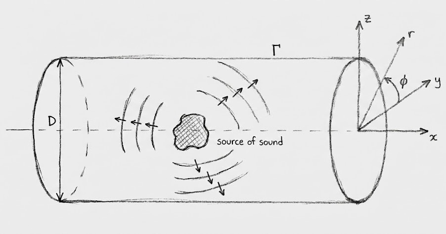
This is where I begin to already take a different approach. In a traditional implementation, you would discretise this surface into panels: triangles or quads, each carrying a centroid, an outward normal, and an area, all as you would with boundary element methods (BEM) for instance. The surface integrals in the FW-H equation are then evaluated panel by panel. This generally works fine, Panels carry connectivity information: which vertex belongs to which face, winding order to determine normal direction, edge adjacency. I’ve never liked panels and index-chasing, its just unfriendly to GPU.
I went a different route. I work with point clouds a lot, the integration surfaces in my solver are going to be point clouds. Point clouds don’t have any connectivity, so to get normals and areas, you need to get a bit complicated with Voronoi or something. I can avoid this entirely though. As already discussed we only need simple shapes, like a cylinder, to enclose our source. This can be derived analytically, A cylinder point gets a radial outward normal and an area weight of ‘r·dφ·dz’, directly from the Jacobian of the cylindrical parameterisation, simple.
from src.surfaces.parametric import cylinder

surface = cylinder(radius=0.5, length=2.0, axis='x', caps=True,
                   n_theta=64, n_z=32)

surface.points.shape   # (3072, 3)
surface.normals.shape  # (3072, 3)
surface.weights.shape  # (3072,)
No connectivity, no winding order, no mesh files and most importantly NO PANELS…Just tensors :)
Getting data onto the surface
So I have a surface defined as a point cloud, and a CFD flow field on a structured Cartesian grid from JAXFLUIDS. The surface points do not sit on grid nodes so we need to do some interpolation.
This is where the k-nearest-neighbour (k-NN) approach comes in (a good friend of mine from work on graph neural nets). For each surface point, I find the k closest CFD cells and blend their values using a Gaussian radial basis kernel wieghting.
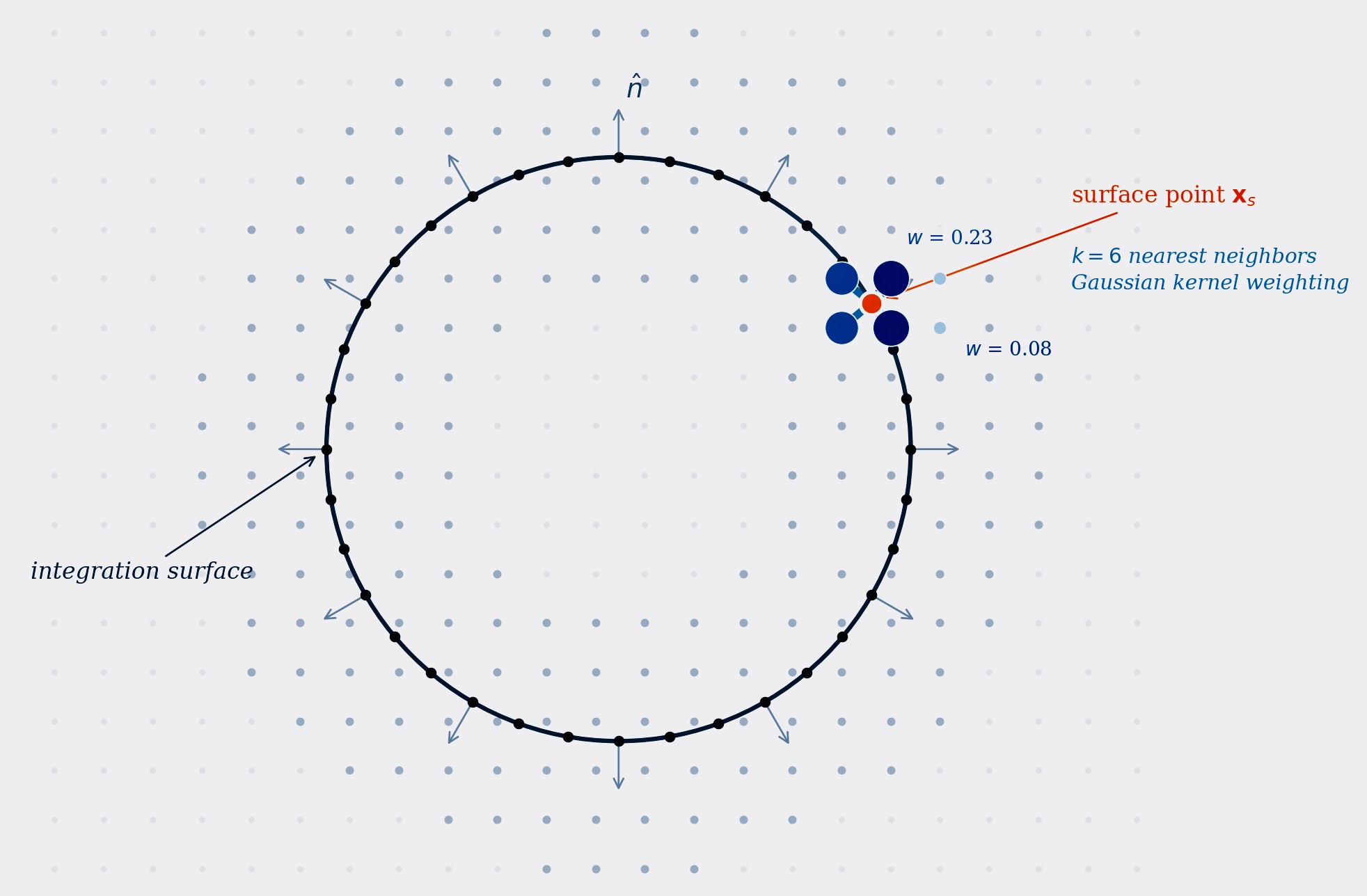
The result is a ScatteredInterpolator that precomputes the neighbour indices and weights once, and then applies them to any field variable with a single gather and weighted sum:
from src.solver.interpolation import ScatteredInterpolator

interp = ScatteredInterpolator.build(
    source_points=cfd_cell_centers,   # (N_cfd, 3)
    target_points=surface.points,     # (N_surface, 3)
    k=8, length_scale='auto'
)

# Map pressure field onto surface, one line per timestep
p_surface = interp(p_cfd)             # (N_surface,)
The two-step pattern is intentional: k-NN search is fast on gpu, this is why I like it, but it will be expensive to run for every time step in a time series, so instead it runs happens once at setup, and then the per-timestep cost is just an indexed lookup and weighted sum (it might not completely work for rotating surfaces however, I have not yet tried this). For static objects in a flow, this will work fine.
The interpolation is where things get interesting from a memory perspective.
Memory and chunking
Remember that the CFD data is going to come from very large grids sizes, typical to LES. The k-NN search requires computing distances between every surface point and every CFD cell
On a Mac with 16 or 32 GB of shared memory, or even on a dedicated GPU with 8-12 GB of VRAM, that full distance matrix is not going to fit and if we brute force this, we will easily go out-of-memory (OOM). This is not an unusual problem size, a well-resolved LES on a domain large enough to enclose a propeller can easily have millions to tens of millions of cells.
N_surface × N_cfd × 4 bytes = 10,000 × 1,000,000 × 4 = 40 GB   ← doesn't fit
chunk:       2,000 × 20,000 × 4                      = 160 MB  ← fits
The solution is chunking: process the target points in batches, compute distances against a chunk of source points, find the k best candidates, merge with the running best, and move on. The chunk sizes are determined at runtime based on how much memory is actually available on whatever device you are running on. On a Mac with MPS, that budget is different from an NVIDIA GPU with dedicated VRAM, so the solver queries available memory and sizes the chunks accordingly.
The merge step is worth a note. As the solver iterates over source chunks, it keeps a running set of the k best neighbours seen so far for each target point. When a new source chunk is processed, it finds the local top-k, concatenates with the running best, sorts, and keeps the overall top-k. This means the full N × M distance matrix never exists in memory, but the result is identical to computing it all at once. chef’s kiss.
This chunker is also dynamic, monitoring memory pressure during the computation. If available memory drops below expectations, it shrinks the chunk size rather than crashing. It only ever shrinks, never grows, which keeps things stable. On mac, memory is unified, so if I want to do something else while it is running, I can easily push to OOM. This can be similar for GPUs that needs to share graphics tasks. It’s not glamorous, actually it was a bit annoying to debug why I was going into memory swaps, but I think it’s the difference between a solver that runs reliably and one that works until it crashes randomly.
Observers
The last piece of geometry before the solver can run is the observers: the locations in space where you want to predict the sound, basically your virtual microphones.
I added a few common arrangements arcs, lines, spheres (for full 3D directivity), and custom layouts. The observer setup is straightforward, but placement matters. The FW-H formulation assumes observers are in the acoustic far-field, so they should be well outside the integration surface. Proximity to the source changes the character of the solution, screams source of error. The final sound pressure is computed at the observers. Because this step works well on GPU, adding more observers costs very little, which helps with denser arrays for error control.
What comes next
What I did not anticipate was the other side quests. I wanted to use custom geometries in JAXFLUIDS, but this needed building out level-set representations from signed distance fields (SDF) and the import pipework was not really there. SDF generation was super slow for large geometry + domain, so I built xSDF, also gpu accelerated. Stories for another post…
You can follow the developement of this FW-H solver here, which I’ve called torchFW-H. A lot has not been pushed to the public repo, but will be there soon. In Part 2, I will get into the actual mathematics of the FW-H formulation, the integral surfaces, the source terms, and how I am approaching the rest of the implementation.
Stay tuned.